Skeleton in the Euclidean closet
Zalán Gyenis
Department of Logic, Jagiellonian University and
Department of Logic, Eötvös University
Abstract
Euclidean Automata have been introduced in Kornai [Kor14a] to model a
phenomenon known as “being in conflicted states”. This brief note gives a
further look on Euclidean Automata and takes the first steps in studying skeleta
and representability and the logical characterization of languages accepted by
Euclidean Automata.
Keywords: Euclidean Automata, Skeleta.
1 Introduction
Euclidean Automata (EA) has been introduced, motivated and further studied in
[Kor14a] and [Kor14b]. EA are slight generalizations of the classical finite state
automata: EA can take continuous parameters as input and are used in [Kor14a] to
analyze the situation of being in a conflicted state. Intuitively, being in a conflicted
state is modeled by an EA not as a single state (of the EA) but rather as a
set of “nondeterministic” states that are represented as overlapping parts of
the input parameter space. Let me recall the precise definition of Euclidean
Automata.
Definition 1.1 ([Kor14b]). A Euclidean automaton (EA) over a parameter space
Σ is defined as a 4-tuple (Q,I,F,α) where Q ⊆ 2Σ is a finite set of states given as
subsets of Σ; I ⊆ Q is the set of initial states; F ⊆ Q is the set of accepting states;
and α : Σ×Q → Q is the transition function that assigns for each parameter setting
v ∈ Σ and each state q ∈ Q a next state α(v,q) that satisfies v ∈ α(v,q). □
In [Kor14a] the EA is called deterministic if q ∩ s = ∅ for different q,s ∈ Q and
complete if ∪q∈Qq = Σ. Throughout we will work with complete EA’s only, the reason is
that for v ∈ Σ -∪q∈Qq the condition v ∈ α(v,q) does not make sense, hence either one
keeps α to be undefined on certain input parameters v or switches to an equivalent EA
with parameter space ∪q∈Qq. For simplicity we assume throughout that the set of initial
states I contains a unique state which we denote by start. If one permits several initial
states he needs to complicate the results accordingly. In applications drawn in
[Kor14a, Kor14b] the alphabet Σ consists of vectors from a continuous parameter space,
typically ℝn, however it also makes sense to consider the definition of an EA when Σ
is a finite set, especially if one considers skeleta of EA’s, as we do in Section
2.
A typical application in [Kor14a] is the heap (Sorites paradox) presented in
the Sainsbury and Williamson [SW95] manner: Consider the line segment [0,1]
colored so that the left-hand region is red, and there is a very fine, continuous,
gradual change of shades reaching the right-hand side region that is colored
yellow. The line is covered by a tiny window that exposes only a small region. We
move the window very slowly starting from the left-hand side towards right and
after each move one is asked about the color of the segment exposed by the
window. But the window is so small relative to the line segment that in no position
can you tell the difference in color between what you can see at the two sides
of the window. It seems that you must call every region red after every move,
and thus you find yourself in the paradoxical situation calling a yellow region
red.
2 Skeleta and representability
Kornai modeled the heap paradox by an EA in a similar manner as we do below (to make
life easier we give a somewhat simplified model, but the differences are inessential for the
sake of the example). Let’s say [0, ] is ‘clearly red’, [
 ,1] is ‘clearly yellow’ and [
 ,
, ] is
this ‘hard to tell, orange’ range. Our EA will have 2 states: red (R) and yellow (Y )
respectively with R = [0,
] is
this ‘hard to tell, orange’ range. Our EA will have 2 states: red (R) and yellow (Y )
respectively with R = [0, ] and Y = [
 ,1]. Note that the two states overlap
exactly in the ‘problematic’ region. Starting from the red state the machine gets
input from the continuous parameter space Σ = [0,1]. The machine is defined as
follows:
,1]. Note that the two states overlap
exactly in the ‘problematic’ region. Starting from the red state the machine gets
input from the continuous parameter space Σ = [0,1]. The machine is defined as
follows:
![{ 2 { 1
α(v,R) = R if v ∈ [0,3] , α (v,Y) = Y if v ∈ [3,1]
Y otherwise. R otherwise.](gyenis6x.png)
In figure:
In the entire fuzzy orangish region [ ,
, ] the model shows hysteresis: if it came from the red
side it will output red, if it came from the yellow side it will output yellow. To get a better
understanding of how EA works, Kornai hints at skeletonizing EA’s. The skeleton of an
EA is defined in [Kor14b] as follows.
] the model shows hysteresis: if it came from the red
side it will output red, if it came from the yellow side it will output yellow. To get a better
understanding of how EA works, Kornai hints at skeletonizing EA’s. The skeleton of an
EA is defined in [Kor14b] as follows.
Definition 2.1 ([Kor14b]). The skeleton of an EA is a standard FSA whose
alphabet corresponds to canonical representatives from each Boolean atom of Q. □
In the deterministic case (where all the states of the EA are disjoint) there is a
correspondence between input letters and automaton states. However, in the
nondeterministic case (where states are not necessarily disjoint) we may not be able to
select distinct canonical representatives for each state (or for the Boolean atoms). In this
case skeleta should be understand as a “subjective EA” (cf. [Kor14b]). The definition
seems a bit vague as it is not completely clear how to chose the so called canonical
representatives (or the subjective representatives), moreover, Q may have no Boolean
atoms (cf. Example 2.4 below). A key for the clarification is the observation that some
inputs are totally indistinguishable no matter what state the machine is in. To obtain
a definition for the general case, fix an EA α : Σ × Q → Q and for v,w ∈ Σ
write
 | (1) |
Then ~ is an equivalence relation on Σ. Moreover it is a congruence of α as for any input
sequences ⟨v1,…,vn⟩ and ⟨w1,…,wn⟩, vi ~ wi implies
After this preparation we can redefine the concept of skeleta as follows.
Definition 2.2. The skeleton of the EA α : Σ × Q → Σ is the standard FSA
α : Σ∕~× Q → Q defined by the equation
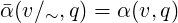
Since ~ is a congruence, α is well-defined. □
If we apply Definition 2.2 to the heap example given above we end up in the finite state
machine figured below, which, unsurprisingly, is exactly the FSA sketched in
[Kor14a]. (Here the input letters r, y and o stand for red, yellow and orange,
respectively)
Observe that Σ∕~ is always finite. This is because the original EA has finitely
many states only, hence we can have a finite number of possibilities not to fulfill
α(v,q) = α(w,q) for input letters v,w. This results in a finite number of equivalence
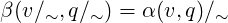
classes of ~. Unfortunately, α is no longer an EA as Q ⁄⊆ 2Σ∕~. It would be handy to
define the skeleton of an EA as another EA over the finite alphabet Σ∕~ by
letting Q∕~ = {q∕~ : q ∈ Q} where q∕~ = {v∕~ : v ∈ q}. However, the automaton
β : Σ∕~× Q∕~→ Q∕~ defined in the obvious manner β(v∕~,q∕~) = α(v,q)∕~ is not
always well defined as the next examples show.
Example 2.3. Below we give an example for an EA the skeleton of which can be
represented as an EA. Let the alphabet (parameter space) be Σ = ℝ and the set of
states is Q = {ℝ,[0,1]}. Let α be the EA figured below defined by the equations
![{
[0,1] if x ∈ [0,1]
α(x,ℝ) = ℝ, α(x,[0,1]) = ℝ otherwise.](gyenis12x.png)
The equivalence relation ~ will have two classes: Σ∕~ = {[0,1], ℝ - [0,1]} = {a,b} and the
skeleton α looks like
Since ℝ∕~ = {a,b} and [0,1]∕~ = {a}, the skeleton is a EA over Q∕~ = {a,b}:
Example 2.4. A small modification on Example 2.3 prevents the skeleton to be
represented by an EA. Here Σ is as before but Q = {ℝ,[0,1],[0,2]}. The EA α is as
figured below on the left-hand side.
The equivalence relation ~ has two classes again: Σ∕~ = {[0,1], ℝ - [0,1]} = {a,b} (note that
elements of [0,2] - [0,1] behave exactly the same way elements of ℝ - [0,1] do). Thus the
skeleton can be figured as above on the right-hand side. Note, however, that
Q∕~ = {{a,b},{a}}, hence the ‘EA representation’
does not make sense as one cannot use the same state differently.
The previous two examples raise the question of representability. In this paper we
could only give a sufficient condition, the general case definitely would require non-trivial
extra work.
Definition 2.5. The EA α : Σ × Q → Q is said to be localizable if for every state
q ∈ Q there is a parameter v ∈ Σ such that v ∈ q -∪r∈Q,r≠qr (that is, v belongs
only to the state q). Localizability means that every state has an eigenparameter, a
parameter which is characteristic of the state. □
In general, a state of a localizable EA can have many different eigenparameters,
thus one rather speaks about the set of eigenparameters associated with a given
state.
Proposition 2.6. Skeleta of localizable EA are isomorphic to EA.
-
- Proof. The idea is that if α is localizable, then ~ extends to a congruence of the
state space Q. That is, if we let Q∕~ = {q∕~ : q ∈ Q} where q∕~ = {v∕~ : v ∈ q},
then the automaton β : Σ∕~× Q∕~→ Q∕~ defined by the equality

will be well-defined. As Q∕~⊆ 2Σ∕~, β will be an EA.
By localizability for every state q there is a parameter vq, an eigenparameter
of q. For two distinct states q and r the corresponding eigenparameters cannot be
~-congruent, because α(vq,q) = q but q does not contain vr, hence α(vr,q)≠q.
The same argument show that α(vq,s) = q for every state s ∈ Q. Therefore all
eigenparameters associated with a given state are equivalent, and each state can be
identified with that equivalence class, that is, there is a bijection between Q and
Q∕~. It follows that α(v∕~,q∕~) = α(v∕~,q). Finally, ~ is defined in such a manner
that α(v,q) = α(w,q) whenever v ~ w. Thus α(v∕~,q) is well-defined, hence β is
well-defined, too. ■
Example 2.3 shows an EA which is not localizable (the state [0,1] does not have an
eigenparameter), still its skeleton can be represented by an EA. This means that
localizability is not necessary for being representable by an EA.
Representation of standard finite state automata can be understood (at least) in two
different ways.
Definition 2.7. Let Ω be a finite alphabet and R a set of states. The FSA
δ : Ω × R → R is representable by an EA if there is EA α over Ω such that α and δ
are isomorphic.
We say that α is representable in the general sense by an EA if there is a
parameter space Σ ⊃ Ω and an EA α over Σ such that α ↾ Ω is isomorphic to δ. □
For an FSA δ : Ω × R → R and a state s ∈ R let us denote by [s]in the set
{v ∈ Ω : (∃p ∈ R)δ(v,p) = s}.
Proposition 2.8. Let δ : Ω × R → R be an FSA with the property that there are
no distinct states s1,s2 ∈ R such that [s1]in = [s2]in. Then δ is representable by an
EA.
-
- Proof. The mapping s
 [s]in is an isomorphism. ■
Example 2.9. Consider the following FSA over the alphabet {v,w,x}.
The sets of incoming edges [s1]in = {v,x} and [s2]in = {w,x} are different, thus after
replacing si by [si]in we get an isomorphic Euclidean automaton.
Unfortunately, the condition in Proposition 2.8 is not necessary: one can construct an
EA that does not satisfy that condition. Here is an easy example. Take a set S and a
partition of S into non-empty sets S1 and S2. Take S to be the alphabet and put
Q = {S,S1,S2} as the set of states. The automaton is defined by α(v,q) = S for any
v ∈ S and q ∈ Q. Then [S1]in = [S2]in = ∅.
Connections with homomorphisms.
In automata theory several different types of homomorphisms between automata are
defined such as state-homomorphism, alphabet-homomorphisms, etc. Since states of
Euclidean automata are subsets of the alphabet, there is a natural way to generalize these
concepts: homomorphisms between Euclidean Automata was defined in [Kor14b] as
follows.
Definition 2.10. A homomorphism from EA α : Σ × Q → Q to another EA
β : Ω × S → S is a mapping h : Σ → Ω such that the following stipulations
hold.
- h(startα) = startβ;
- h extends to a mapping h : Q → S in the natural way;
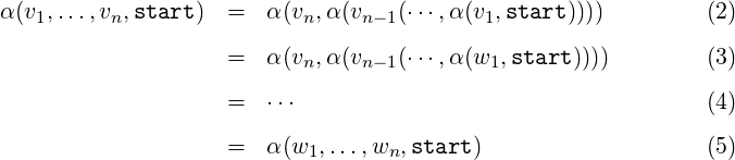
- h
 α(v1,…,vn,start)
 = β(h(v1),…,h(vn),start).
□
By Proposition 2.6 skeleta of localizable EA remain Euclidean: For a localizable EA
α : Σ × Q → Q the congruence ~ defined by (1) extends to a congruence of the state
space Q. That is, if we let Q∕~ = {q∕~ : q ∈ Q} where q∕~ = {v∕~ : v ∈ q}, then the
automaton β : Σ∕~× Q∕~→ Q∕~ defined by the equality
is an EA. Let us denote this β by  . It is very easy to check (cf. the proof of Proposition
2.6), that
. It is very easy to check (cf. the proof of Proposition
2.6), that  and the skeleton α defined in 2.2 are isomorphic. Therefore we will call
  also
a skeleton of α.
also
a skeleton of α.
Now, if α is localizable, then  is a homomorphic image of α. For, write h(v) = v∕~,
where ~ is the congruence defined by (1). The first two items of Definition 2.10 follows
from the proof of Proposition 2.6 and the third item is the very definition of
is a homomorphic image of α. For, write h(v) = v∕~,
where ~ is the congruence defined by (1). The first two items of Definition 2.10 follows
from the proof of Proposition 2.6 and the third item is the very definition of  as
h
as
h α(v,q)
 = α(v,q)∕~ =
  (v∕~,q∕~).
An important consequence is that localizable EA’s are categorical objects in the sense
that the class of all such automata is closed under the homomorphism introduced in
Definition 2.10, and skeleta form a closed subcategory of the category of all localizable
EA.
3 Languages accepted by EA
In this section we turn to a logical characterization of the languages that can be accepted
by EA. Let δ : Ω × R → R be a standard FSA. The language of α is the set Lα ⊆ Ω*
defined as

This definition clearly makes sense even if Ω is infinite. Therefore one can define without
any difficulty when a Euclidean automata α : Σ × Q → Q accepts a language L ⊆ Σ*: if
and only if L = Lα.
This definition, however, may not be satisfactory enough when Σ is infinite. The
reason is that one might like to say that the skeleton of an EA accepts the same language
as the original EA when restricted to the language of the skeleton. More precisely one can
consider the skeleton acting on a subset of the original alphabet: pick a representative
from each of the equivalence class of the alphabet of the skeleton. Then the skeleton and
the original EA shows the same behavior on each input string. This motivates the next
definition.
Definition 3.1. Suppose α : Σ×Q → Q is an EA, where Σ is allowed to be infinite.
Let Ω ⊆ Σ be a finite subalphabet and L ⊆ Ω* a language. Then α is said to accept
L in the general sense if Lα ↾ Ω* = L. □
Proposition 3.2. Each regular language can be accepted in the general sense by
an EA.
-
- Proof. Let L be a regular language over Ω and δ : Ω×R → R the FSA that accepts
L. By adding new letters to Ω one can reach that in this expanded language (denote
it by Σ) the FSA satisfies [s]in≠[s′]in for all states s,s′∈ R by defining the action of
the new letters carefully. The resulting FSA is representable by an EA α applying
Proposition 2.8. It is clear that Lα ↾ Ω* = L. The proof reveals that more is true: any
language accepted by an FSA over a possibly infinite alphabet can also be accepted
in the general sense by an EA. If Ω is finite then Σ can chosen to be finite; otherwise
they can have the same infinite cardinality. ■
It is obvious that every language accepted by an EA is regular (because EA are special
FSA), thus the question of which languages are accepted in the general sense is settled.
The cheat here is that we are allowed to enlarge the alphabet. Is it true that keeping the
same alphabet, for every FSA δ : Σ × R → R there is a EA α : Σ × Q → Q such that
Lδ = Lα? If the alphabet is finite, then the answer obviously is ‘no’. This is because over a
finite alphabet Σ one can define at most finitely many EA as the set of states Q
should be a subset of 2Σ which is still finite. But what about the infinite case
where one can have any finite number of states? The answer is still ‘no’ but for
different reasons: the language that contains words having odd length (over
any alphabet Σ) can be accepted by an FSA but cannot be accepted by any
EA.
Example 3.3. No EA can accept the language containing words having odd length.
-
- Proof. The language L = {w ∈ Σ* : |w| is odd } is accepted by the FSA figured
below.
Suppose there is an Euclidean automaton (Q,I,F,α) that accepts L. The first input
letter v1 can be any letter from Σ, hence after the first transition α(v1,start) = q1, the
resulting state should q1 should contain v1 by Euclideanity. This means q1 = Σ. The
second letter v2 is also arbitrary, hence after the second transition α(v2,q1) = q2
we get similarly that q2 = Σ. This means q1 = q2 and in fact continuing the
argument one get the conclusion that there can be only one state Q = {Σ}.
But such an EA accepts all strings and not just the ones having odd length.
■
It is known that regular languages are exactly the languages that can be
defined in monadic second order logic [Bu60, El61]. Let us recall some of the basic
definitions to make everything clear. Let Σ be an alphabet (possibly infinite) and let
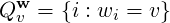
w = ⟨w1,…,wn⟩ be a word in Σ*. Such a word can be represented by the relational
structure

called the word model for w, where < w is the usual ordering on the domain of w and
Qvw are unary predicates collecting for each letter v ∈ Σ those letter positions of w which
carry v:
The corresponding first-order language FO(Σ) has variables x,y,… and built up the
grammar

The language defined by a formula φ is Lφ = {w ∈ Σ* : w φ}, where the satisfaction
relation
φ}, where the satisfaction
relation  is defined in the usual way. For example the language where “every a is
immediately followed by a b” can be defined by the formula
is defined in the usual way. For example the language where “every a is
immediately followed by a b” can be defined by the formula

where y = x + 1 has the usual definition x < y ∧¬∃z(x < z ∧ z < y). A non-example
could be L = {a2n : n ∈ ℕ} which is not expressible by a first order formula
[Esp12].
Monadic second order logic MSO(Σ) is an extension of first order logic with variables
X,Y,… ranging over sets of elements of models. The corresponding atomic formulas
X(x) are also introduced with the intended meaning “x belongs to X”. Clearly
MSO(Σ) is more expressive than FO(Σ) but not vice-versa as the next theorem
shows:
Theorem 3.4 (Büchi [Bu60], Elgot [El61]). A language (over a finite alphabet) is
recognizable by a finite state automaton if and only if it is MSO(Σ)-definable, and
both conversions, from automata to formulas and vice versa, are effective.
Thus, regular languages are exactly the monadic second order definable languages.
However, examples suggests that languages accepted by Euclidean automata are first
order definable:
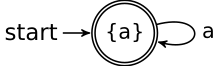
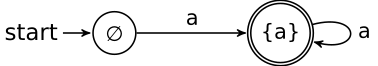
Example 3.5. For Σ = {a} we must have Q ⊆{∅,{a}} and thus there are exactly two
non-isomorphic EA, figured below
The languages accepted by the automata are L1 = {an : n ≥ 0} and L2 = {an : n ≥ 1}. Both
languages are definable in the language FO(Σ), respectively by the formulas ∀xQa(x) and
∃xQa(x) ∧∀xQa(x).
Example 3.6. For Σ = {a,b} the number of variations is larger than before
as Q ⊆ {∅,{a},{b},{a,b}} gives more possibilities. We will not draw all the
non-isomorphic EA’s here, but one can check easily that the languages that can be
accepted by EA over Σ are of the form “all sequences of a’s and b′s + if we wish we
can prescribe the first and last letter”. For example such an L can contain all words
starting with an a. In any case a FO(Σ)-characterization can be easily given. (As
we prove next that languages accepted by EA are first order definable, we omit the
details of the rather painstaking checking of this claim).
Indeed, we prove that languages accepted by Euclidean automata are FO-definable.
Proposition 3.7. For every finite alphabet Σ there is a corresponding first order
language FO such that each language accepted by an Euclidean automaton can be
defined by a FO-formula.
-
- Proof. Assume (Q,I,F,α) is a Euclidean automaton over the finite parameter space Σ.
Take the first order language FO(Σ) described above and expand this language by new
unary predicates Ri for i < 2|Σ|. We have to find a first order formula that expresses in
any given word model w that α accepts w. The formula in question will state the
existence of a successful run of the EA. As α has finitely many state, we can enumerate
them by Q = {qi : i < 2|Σ|}. Each state qi of the EA will be encoded by the
predicate Ri. We need to express the followings: (1) in each turn the machine
can be only in one state; (2) the starting state is q0; (3) if we are in position x
and the next position is y, then we applied one of the letters, i.e. for one of the
v ∈ Σ we have Qv(x), and thus the next state should be the one prescribed by
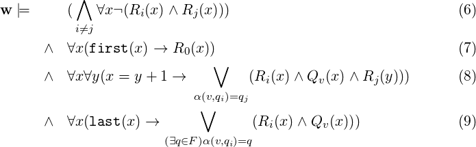
α(v,qi) = qj; (4) the last position is a final state. Thus α accepts w if and only if
Since the empty word satisfies this sentence, if α does not accept the empty word, then a
corresponding clause such as ∃x(x = x) should be added. first(x) and last(x) are
respectively the formulas ¬∃y(y < x) and ¬∃y(x < y). ■
If the alphabet Σ is not finite, then a similar argument shows that languages accepted
by EA can be defined by first order formulas that are allowed to contain infinite
disjunctions having an infinite vocabulary (i.e. we use the logic FO∞ω).
Recall that finiteness is a property that cannot be expressed in first order logic.
Indeed, by the compactness theorem if a formula holds in all finite models, then it should
also hold in an infinite model. This can be seen as one of the main reasons why languages
that can be accepted by finite state automata cannot be defined in first order
logic (and one needs monadic second order logic). Even if the alphabet is fixed,
an FSA can have an arbitrary finite number of states and we do not have any
control, in terms of first order logic, over the number of states. As we already seen,
there are only finitely many EA over a finite alphabet. That is, if we fix the
alphabet, then there is a fixed upper bound on the possible number of states,
depending only on the size of the alphabet. This allows us to bypass the problem of
non-definability of finiteness: using first order logic it is easy to define models
having size at most n, for a fixed finite number n. This is the key for Proposition
3.7.
As we already mentioned, there are only finitely many EA over a finite alphabet.
Therefore not every first order definable language can be accepted by an EA (there are
infinitely many first order definable languages). Then what is the logic that is exactly as
expressible as Euclidean automata? As the number of states is limited, the set of EA do
not have any extensive closure property (such as closed under direct product,
unions, etc). This suggests use the vague idea that EA are not logical in the sense
of expressibility. Of course it is not clear how to define ‘logicality’ in a precise
manner.
Acknowledgement
I am grateful to the Reviewer for his/her careful reading of the manuscript and the
helpful suggestions. I wish to acknowledge the Premium Postdoctoral Grant of the
Hungarian Academy of Sciences hosted by the Logic Department of the Loránd Eötvös
University.
References
[Bu60] Büchi, J.R., (1960) Weak second-order arithmetic and finite automata.
Z. Math. Logik Grundl. Math. 6, pp. 66–92.
[El61] Elgot, C.C., (1961) Decision problems of finite automata design and
related arithmetics. Trans. Amer. Math. Soc. 98, pp. 21–52.
[Kor14a] Kornai, András (2014) Euclidean Automata. In: Implementing Selves
with Safe Motivational Systems and Self-Improvement, 2014.03.24–2014.03.26,
Los Angeles, USA.
[Kor14b] Kornai, András (2014) Finite automata with continuous input. In: S.
Bensch and R. Freund and F. Otto (eds.) Short Papers from the Sixth Workshop
on Non-Classical Models of Automata and Applications.
[SW95] Sainsbury, M., and Williamson, T. (1995) Sorites. In Hale, B., and
Wright, C., eds., Blackwell Companion to the Philosophy of Language.
Blackwell.
[Esp12]
Esparza, Javier (2012) Automata theory, an algorithmic approach. Lecture
notes, http://www.fi.muni.cz/usr/kretinsky/MSO_Javier_Esparza.pdf,
Accessed: Aug 21, 2017.