Building word embeddings from dictionary definitions

We present an experimental method for mapping English words to real-valued vectors using entries of a large crowd-sourced dictionary. Intuition tells us that most of the information content of the average utterance is encoded by word meaning (Kornai (2010) posits 85%), and mappings of words to vectors (commonly known as word embeddings) have become a core component of virtually all natural language processing (NLP) applications over the last few years. Embeddings are commonly constructed on the basis of large corpora, approximating the semantics of each word based on its distribution. In a set of pilot experiments we hope to demonstrate that dictionaries, the most traditional genre of representing lexical semantics, remain an invaluable resource for constructing formal representations of word meaning.

1 Background

Nearly all common tasks in natural language processing (NLP) today are performed using deep learning methods, and most of these use word embeddings – mappings of the vocabulary of some language to real-valued vectors of fixed dimension – as the lowest layer of a neural network. While many embeddings are trained for specific tasks, the generic ones we are interested in are usually constructed with the objective that words with similar distributions (as observed in large corpora) are mapped to similar vectors. In line with the predictions of the distributional hypothesis, this approach causes synonyms and related words to cluster together. As a result, these general-purpose embeddings serve as robust representations of meaning for many NLP tasks; however, their potential is necessarily limited by the availability of data. Lack of training data is a major issue for all but the biggest languages, and not even the largest corpora are sufficient to learn meaningful vectors for infrequent words. Lexical resources created manually, such as monolingual dictionaries, may be expensive to create, but crowdsourcing efforts such as Wiktionary or UrbanDictionary provide large and robust sources of dictionary definitions for large vocabularies and – in the case of Wiktionary – for many languages.

Recent efforts to exploit dictionary entries for computational semantics include a semantic parser that builds concept graphs from dependency parses of dictionary definitions (Recski, 2016; Recski, to appear) and a recurrent neural network (RNN) architecture for mapping definitions and encyclopaedia entries to vectors using pre-trained embeddings as objectives (Hill et al., 2016). In this paper we construct embeddings from dictionary definitions by encoding directly the set of words used in some definition as the representation of the given headword. We have shown previously (Kornai et al., 2015) that applying such a process iteratively can drastically reduce the set of words necessary to define all others. The extent of this reduction depends on the – possibly non-deterministic – method for choosing the set of representational primitives (the defining vocabulary). The algorithm used in the current experiment will be described in Section 2. Embeddings are evaluated in Section 3, Section 4 presents our conclusions.

2 Word vectors from dictionary definitions

In this research, we eschew a fully distributional model of semantics in favor of embeddings built from lexical resources. At first glance, the two approaches seem very different: huge corpora and unsupervised learning vs. a hand-crafted dictionary of a few hundred thousand entries at most. Looking closer, however, similarities start to appear. As mentioned previously, generic (“semantic”) embeddings are trained in such a way that synonyms and similar words cluster together; not unlike how definitions paraphrase the definiendum into a synonymous phrase (Quine, 1951). The two methods thus can be viewed as two sides of the same empirical coin; we might not fully go against Quine then when we “appeal to the nearest dictionary, and accept the lexicographer’s formulation as law”. Representing (lexical) semantics as the connections between lexical items has a long tradition in the NLP/AI literature, including Quillian’s classic Semantic Memory Model (Quillian, 1968), widely used lexical ontologies such as WordNet (Miller, 1995) and recent graph-based models of semantics such as Abstract Meaning Representations (Banarescu et al., 2013) and 4lang (Kornai, 2012; Recski, to appear).

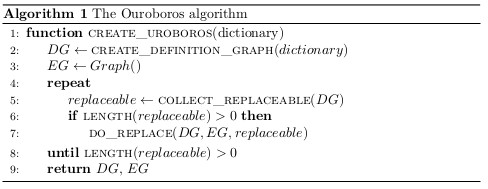
In the model presented below, word vectors are defined not by count distributions (as in e.g. Pennington et al. (2014)), but by interconnections between words in the dictionary. For the purpose of this paper, we chose the English Wiktionary¹ as the basis of our embedding, because it is freely available; however, the method would work on any monolingual dictionary. The word vectors are computed in three steps.

First, we preprocess the dictionary and convert it into a formal structure, the definition graph: a directed graph whose vertices correspond to headwords in the dictionary. Two vertices A and B are connected by an edge A ← B if the definition of the head contains the tail, e.g. A: B C D. Definition graphs can be weighted and unweighted. In the former, each vertex distributes the unit weight among its in-edges equally; in the latter, each edge has a weight of 1. Continuing the previous example, the edges from B, C and D to A have a weight of in the weighted graph and 1 in the unweighted one.

Next, an iterative algorithm is employed to find an “Ouroboros” set of words, which satisfies two conditions:

1. the whole vocabulary can be defined in terms of it, i.e. all directed paths leading to a word in the definition graph can be traced back to the Ouroboros set
2. it can define itself, so no words outside the set appear in the definitions of its members (we call this self-containedness the ouroboros property).

The idea that a small set of primitives could be used to define all words in the vocabulary is not new (Kornai, in press); several such lists exist. The most relevant to the current work is probably the Longman Defining Vocabulary (LDV), used exclusively in the definitions of earlier versions of the Longman Dictionary of Contemporary English (LDOCE) (Bullon, 2003). The LDV is not minimal, and in previous work it served as our starting point to reduce the size of the essential word set as much as possible (Kornai et al., 2015). Here we chose a different approach, not least because no such list exists for Wiktionary.

Finding the Ouroboros set would be easy if the definition graph was a DAG. However, due to the interdependence of definitions in the dictionary, the graph contains (usually many) cycles. Our algorithm deals with this by choosing a “defining” node in each cycle, and collecting these in a set. Then, all arrows from outside of the set to inside it are removed. It is clear that this set is defining, as every non-member vertex is reachable from the nodes in it. Furthermore, after the removal of inbound edges, the set satisfies the second condition and therefore it is an Ouroboros.

Trivially, the whole dictionary itself is an Ouroboros set, provided that dangling edges (corresponding to words in definitions that are themselves not defined in the dictionary) are removed from the definition graph² . Needless to say, we are interested in finding the smallest possible (or at least, a small enough) set that satisfies the property.

Mathematically inclined readers might recognize our Ouroboros as the feedback vertex set of the definition graph. In the remainder of this paper, we shall stick to the former (perhaps inaccurate) name, as it also hints at the way it is generated – see section 2.2. Furthermore, elements of the set shall be referred to – perhaps even more incorrectly than the singular term – with the plural form, ouroboroi.

In the final step of the algorithm, the vertices of the definition graph are mapped into real valued vectors in ℝⁿ, where n is the size of the Ouroboros set. The vectors that correspond to the ouroboroi serve as the basis of the vector space; they are computed from the structure of the Ouroboros subgraph. Other words are assigned coordinates in this space based on how they are connected to the ouroboroi in the definition graph.

It is worth noting that in our case, the dimensionality of the embedding is dictated by the data; this is in sharp contrast to regular embeddings, where n is a hyperparameter.

The steps are explained in more detail below.

2.1 Preprocessing the dictionary

A dictionary is meant for human consumption, and as such, machine readability is, more often than not, an afterthought. Wiktionary is no exception, although its use of templates makes parsing a bit easier. We used the English dump of May 2017, and extracted all monolingual entries with the wiktionary_parser tool from the 4lang library³ . The definitions are then tokenized, lemmatized and tagged for POS by the corresponding modules of the Stanford CoreNLP package (Manning et al., 2014).

At a very basic level, tokenization is enough to produce a machine readable dictionary. However, further transformations were applied to the dictionary to improve recall and decrease its size by removing irrelevant data, as well as to correct inconsistencies in how it was compiled. Raw word forms generally give low recall because of the difference in inflection between definienda and definientia. To solve this problem, we employed two essential techniques from information retrieval (IR): lemmatization and lowercasing. Our aim with the dictionary is to build a definition graph of common words. Looking at the dictionary from this angle, it is clear that it contains a large amount of irrelevant data.

• multiwords: Wiktionary has entries for multiword units, such as expressions and noun compounds. While this poses no problems for the algorithm described below, currently we have no means to evaluate such lexical units.
• proper nouns: proper nouns often cluster into strongly connected groups, such as mythologies (Étaín, Midir and the Dagda, amongst others, represent Ireland) or country-capital pairs (e.g. Dehradun and Uttarakhand from French India). Each such group inevitably “delegates” one of its members to the ouroboros, increasing its size for negligible gains.
• punctuation: punctuation marks clearly have no role on the semantic level; on the syntactic side, our BOW approach renders them superfluous.
• stopwords: similarly to punctuation, function words bring very little to the table; removing them is a common practice in IR.

We created a dictionary file for every combination of the transformations described above. Proper nouns and punctuation were filtered by their POS tags; stopwords according to the list in NLTK (Bird et al., 2009). In case of the latter two, not only were the tokens removed from the definitions, but their entries were also dropped. Table 1 lists the most important versions, as well as the effect of the various filtering methods on the size of the vocabulary and the Ouroboros of the resulting dictionary. It can be seen that lowercasing and lemmatization indeed increase the recall, and that multiwords and proper nouns make up about one third of the dictionary. The effect on the size of the Ouroboros seems more incidental; it is certainly not linear in the change in vocabulary size.

The linguistic transformations above have been straightforward. However, we are also faced with lexicographical issues that require further consideration. The first of these concerns entries with multiple senses: homonymous and polysemous words. While the former needs no justification, the interpretation of polysemy, as well as the question of when it warrants multiple definitions, is much debated (see e.g. Bolinger (1965) and Kirsner (1993) and the chapter on lexemes in Kornai (in press)). Aside from any theoretical qualms one may have, there is also a practical one: even if the different senses of a word are numbered, its occurrences in the definitions are not, preventing us from effectively using this information. Therefore, we decided to merge the entries of multi-sense words by simply concatenating the definitions pertaining to the different senses.

The second problem is inconsistency. One would logically expect that each word used in a definition is itself defined in the dictionary; however, this is not the case. Such words should definitely be added to the ouroboros, but having no definition themselves, would contribute little to its semantics. As such, we eliminated them with an iterative procedure that also deleted entries whose definition became empty as a result. The procedure ran for 3–4 iterations, the number of removed entries / tokens ranging from 5342 / 912,373 on the raw dictionary to 707 / 125,509 on the most heavily filtered version.

Finally, in some entries, the definiens contains the definiendum. Since the presence or absence of these references – an artifact of the syntax of the language the definition is written in, not the semantics of the word in question – is arbitrary, they were removed as well.

2.2 The Ouroboros

Once the dictionary is ready, the next step towards the embedding is creating the Ouroboros set, which will serve as the basis of the word vector space. The Ouroboros is generated by an iterative algorithm that takes the definition graph as input and removes vertices at each iteration. The vertex set that remains at the end is the Ouroboros. A high-level pseudocode of the algorithm is included at the end of this section.

An iteration consists of two steps. In the first, we iterate through all words and select those that can be replaced by their definition. A word can be replaced if the following conditions hold:

1. no other words connected to the word in question in the definition graph (via both in- or out-edges) have been marked for replacement;
2. the vertex that corresponds to the word has no self-loop.

The first condition is simply a way of preventing race conditions in the replacement process. The second one, however, calls for some explanation. As we made sure that no definition contains its headword in the dictionary, initially, the definition graph contains no self-loops. However, as more and more words are removed, self loops start to appear. This is also our final stopping condition: the algorithm exits when all remaining vertices are connected to themselves. One can look at this condition as a way of saying that a word in the Ouroboros cannot be defined solely in terms of other words – in a way, it eats its own tail.

The second step performs the actual replacement. It removes the vertices marked by the first step, and connects all of their direct predecessors in the graph to their directs successors. In the weighted version, the weights are updated accordingly: the weight of a new edge will be equal to the product of the weights of the two edges it replaces. Figure 1 illustrates the replacement procedure with an example.

This step is also responsible for building the embedding graph. At first, the graph is empty. Each vertex removed by the algorithm, together with its in-edges, is added to it. By the time the algorithm stops, all vertices will have been added to the embedding graph. It is easy to see that this graph is a DAG, with the ouroboroi as its sources: what the whole algorithm effectively does is decrease the size of the cycles in the definition graph, vertex-by-vertex and edge-by-edge. The cycles never disappear completely, but become the self loops that mark the Ouroboros set. It follows then, that the Ouroboros contains at least one vertex and one edge (the self loop) from each cycle in the original definition graph and thus the embedding graph is free of (directed) cycles.

This algorithm can be tuned in several ways. The attentive reader might have noticed that the order in which the words are evaluated in the first step strongly determines which end up as replaceable. Several strategies were considered, including alphabetical and random order, shortest / longest, or rare / most common word (in definitions) first. Not surprisingly, rare words first performed best: this agrees with the intuition that the “basis” for the embedding should mostly contain basic words. Consequently, all numbers reported in this paper were attained with the rare first strategy.

We also experimented with decreasing the size of the embedding graph by deleting edges below a certain weight threshold; this is the equivalent of magnitude-based pruning methods in neural networks (Hertz et al., 1991). However, the performance of the embeddings created from pruned and unweighted graphs lagged behind those created from weighted ones. Hence, we used the latter for all experiments.

2.3 The Embedding

This section describes the algorithm that takes as its input the ouroboros and embedding graphs and produces a word embedding. First, the basis of the vector space is computed. Since our goal is to describe all words in terms of the Ouroboros, the vector space will have as many dimensions (denoted with D) as there are vertices in the Ouroboros graph. Each coordinate corresponds to a word; the mapping is arbitrary, and we opted for alphabetic order. The word vectors for the ouroboroi (the first D rows of the embedding) are chosen to be the basis vectors of the vectors space.

The basis vector for an Ouroboros word w, however, can be calculated in two ways:

1. Ouroboros-as-coordinates (OAC): as a sparse vector, where the only nonzero coordinate is the one that corresponds to the word itself. The first D rows of the embedding thus form the identity matrix.
2. Ouroboros-as-vectors (OAV): as a vector whose nonzero coordinates correspond to the direct predecessors of w in the ouroboros graph. The values of the coordinates are the weights of the edges between its predecessors and w.

The two variants have opposing properties. OAV is much denser, which might bring words much closer in the semantic space than they really are, introducing “false semantic friends”. OAC, on the other hand, is so sparse that the similarity of two Ouroboros words is always zero. This property might be useful if our algorithm was guaranteed to find the most semantically distributed feedback vertex set; however, no such guarantee exists. Since it is hard to choose between the two based solely on theoretical grounds, both variants are evaluated in the next chapter.

The vectors for the rest of the words are computed from the embedding graph. The graph is sorted topologically, with the ouroboroi at the beginning. The algorithm iterates through the words. The vector of a word w is set to be the weighted sum of the vectors of its direct predecessors in the embedding graph:

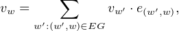
where e_(i,j) is the weight of the edge between i and j. The topological sort ensures that by the time we arrive to w, the vectors for all w′s have already been calculated.

More by accident than design, we also created a third embedding beside OAC and OAV. Here the basis is taken from OAV, but the rest of the vectors are the same as for OAC; accordingly, we named it Chimera (CHI). While the construction of this embedding is mathematically incorrect, it performed unexpectedly well, so we included it in the evaluation alonside OAC and OAV.

3 Evaluation

The algorithm presented in Section 2 creates word embeddings, i.e. mappings from the vocabulary of a dictionary dataset to real-valued vectors of fixed dimension. This section will present two sets of experiments, both of which indicate that the distance between pairs of word vectors is a meaningful measure of the semantic similarity of words. In Section 3.1 we will use two semantic similarity benchmarks for measuring semantic similarity of English word pairs to evaluate and compare our word embeddings. Section 3.2 presents a qualitative, manual analysis of each embedding that involves observing the set of words that are mapped to vectors in the immediate vicinity of a particular word vector in the embedding space.

3.1 Benchmark performance

The embeddings were evaluated on two benchmarks: SimLex-999 (Hill et al., 2015) and WS-353 (Finkelstein et al., 2002).

SimLex is the new standard benchark for the task of measuring the semantic similarity of English word pairs. It contains 999 word pairs, each annotated with a gold standard similarity score, the average of scores given by human annotators. Performance of systems is measured as the Spearman correlation between a system’s scores and the gold standard scores. State of the art systems achieving correlation scores in the 0.7-0.8 range (Mrkšić et al., 2016; Recski et al., 2016) combine multiple word embeddings and lexical resources, other competitive systems use word embeddings customized for the task of measuring word similarity (Schwartz et al., 2015; Wieting et al., 2015). General-purpose embeddings typically achieve a correlation in the 0.1-0.5 range; scores for some commonly used models are shown in Table 2.

The WS-353 dataset contains 353 word pairs. It was originally devised to quantify any kind of semantic association: both similarity and relatedness. Here we use the subset that targets the former, selected by Agirre et al. (2009). Similarly to Simlex, performance is measured by Spearman’s ρ. WS-353 has been around longer than Simlex, and various corpus- (Gabrilovich and Markovitch, 2007; Halawi et al., 2012) and knowledge-based methods (Hassan and Mihalcea, 2011) have been evaluated against it; the current state-of-the-art, 0.828 was achieved by a hybrid system that also makes use of word embeddings (Speer et al., 2017).

We evaluate various versions of our ouroboros-embeddings on both datasets. Results are presented in Table 3. Top scores on Simlex are just above 0.2, which outperforms Huang, but falls short of GloVe and Word2Vec by a similar margin. On the much easier WS-353 dataset, even our best result is below that of the competition. Nevertheless, these results confirm that our method yields vectors that are at least comparable to other general-purpose embeddings.

An early observation is that embeddings created using the OAV condition (see Section 2.3) perform considerably worse than those built with the OAC condition. The most surprising part is the performance of the CHI embedding: while it tails behind the other two methods on Simlex, it improves dramatically when stopwords are filtered (the last two rows), to the extent that it becomes the best method on both datasets.

In order to gain further insight into how the three embeddings behave differently, we devised a further experiment based on the all embedding. The word pairs in the evaluation datasets have been divided into three groups, depending on how many of the two words are ouroboroi. Table 4 presents the results. Unsurprisingly, the numbers for CHI equal to OAV when both words are in the Ouroboros and to OAC when neither is. Perhaps predictably, our concerns about both OAC and OAV have been confirmed by the results: the orthogonal OAC basis breaks down when both words in a pair are in it, while the over-dense OAV fails to quantify the similarity of out-of-basis pairs. CHI, on the other hand, manages to be the “best of both worlds”, at least as far as the first and the last row is concerned. Its exceptional performance in the middle row (in italics) is perplexing, because this is the point where OAV basis vectors are measured against OAC vectors; where the snake meets the lion, so to speak. Unfurling this mystery is left as future work.

Both SimLex and WS-353 contain pairs of frequent words. Our hope is that in the next section our method will show its strength on infrequent words that cause trouble for distributional models that are limited by the amount of training data available.

3.2 Nearest neighbors

As mentioned in Section 1, we expect our embeddings to yield meaningful representations even for infrequent words that pose a problem for distributional approaches. We have no knowledge of reliable datasets containing the semantic similarity of infrequent words, a quantitative analysis is therefore not possible. A more subjective method to evaluate whether the angle between word vectors is proportional to semantic similarity is to observe vectors in the immediate vicinity of a particular vector to see whether they are semantically related to the word corresponding to that vector. Our experiment involves examining the nearest neighbors of vectors corresponding to a small sample of infrequent words in our least noisy ouroboros-embedding (using all filtering steps on the Wiktionary data) and a large, publicly available embedding trained using GloVe on 840 billion words of raw English text and containing vectors for 2.2 million words.

To create a sample of infrequent English words, we used a word frequency list constructed from the UMBC Webbase Corpus (Han et al., 2013). To extract words that are in English, correctly spelled, and can be expected to appear in a dictionary, we matched the list against the full vocabulary used in a late draft version of (Kornai, in press), which we know to contain many infrequent words. After manually excluding from the resulting list technical words related to mathematics or linguistics, we kept the five least frequent ones for the purposes of the current experiment. The five words, along with their definitions in Wiktionary, are shown in Table 5. For both the uroboros and GloVe embeddings we extracted the nearest neighbors of each of the five words in our sample. Tables 6 and 7 show for each word the top two neigbors in the uroboros and GloVe embeddings, respectively. We also include Wiktionary definitions of these neighbor words, where available.

Even such a small and non-representative sample of infrequent English words is sufficient to exemplify some of the issues that arise when representing infrequent words with distributional models. Typos of more frequent words may dominate the total number of occurrences in a corpora: compter and hinny are clearly represented by the GloVe embedding as alternative forms of computer and hiney, respectively. Neighbors of the other three sample words in the GloVe embedding are seemingly random. Meanwhile, in 4 out of the 5 example cases, uroboros maps rare words into the vicinity of highly related lexemes.

4 Conclusion

In this work, we examined the possibility of creating word embeddings from a dictionary. While the performance of our embedding in the word similarity task lags behind those obtained by prediction-based methods, it is perhaps better suited to find relevant neighbors of rare words.

In future work, we hope to iron out the sparsity/density problem that is, in part, responsible for the lackluster similarity scores. Another avenue of research we intend to pursue is to consolidate prediction- and dictionary-based embeddings into a hybrid model that combines the advantages of both.

References

Agirre, Eneko, Enrique Alfonseca, Keith Hall, Jana Kravalova, Marius Paşca, and Aitor Soroa (2009). “A study on similarity and relatedness using distributional and Wordnet-based approaches”. In: Proceedings of Human Language Technologies: The 2009 Annual Conference of the North American Chapter of the Association for Computational Linguistics. Association for Computational Linguistics, pp. 19–27.

Banarescu, Laura et al. (2013). “Abstract Meaning Representation for Sembanking”. In: Proceedings of the 7th Linguistic Annotation Workshop and Interoperability with Discourse. Sofia, Bulgaria: Association for Computational Linguistics, pp. 178–186.

Bird, S., E. Klein, and E. Loper (2009). Natural language processing with Python. O’Reilly Media.

Bolinger, Dwight (1965). “The atomization of meaning”. In: Language, pp. 555–573.

Bullon, Stephen (2003). Longman Dictionary of Contemporary English 4. Longman.

Collobert, Ronan and Jason Weston (2008). “A Unified Architecture for Natural Language Processing: Deep Neural Networks with Multitask Learning”. In: Proceedings of the 25th International Conference on Machine Learning. ICML ’08. Helsinki, Finland: ACM, pp. 160–167.

Finkelstein, Lev, Evgeniy Gabrilovich, Yossi Matias, Ehud Rivlin, Zach Solan, Gadi Wolfman, and Eytan Ruppin (2002). “Placing Search in Context: The Concept Revisited”. In: ACM Transactions on Information Systems 20(1), pp. 116–131.

Gabrilovich, Evgeniy and Shaul Markovitch (2007). “Computing semantic relatedness using wikipedia-based explicit semantic analysis”. In: IJcAI. Vol. 7, pp. 1606–1611.

Halawi, Guy, Gideon Dror, Evgeniy Gabrilovich, and Yehuda Koren (2012). “Large-scale learning of word relatedness with constraints”. In: Proceedings of the 18th ACM SIGKDD international conference on Knowledge discovery and data mining. ACM, pp. 1406–1414.

Han, Lushan, Abhay L. Kashyap, Tim Finin, James Mayfield, and Jonathan Weese (2013). “UMBC_EBIQUITY-CORE: Semantic Textual Similarity Systems”. In: Second Joint Conference on Lexical and Computational Semantics (*SEM). Atlanta, Georgia, USA: Association for Computational Linguistics, pp. 44–52.

Hassan, Samer and Rada Mihalcea (2011). “Semantic Relatedness Using Salient Semantic Analysis.” In: AAAI.

Hertz, John A, Anders S Krogh, and Richard G Palmer (1991). Introduction to the Theory of Neural Computation. Vol. 1. Redwood City, CA: Addison-Wesley.

Hill, Felix, Roi Reichart, and Anna Korhonen (2015). “Simlex-999: Evaluating semantic models with (genuine) similarity estimation”. In: Computational Linguistics 41.4, pp. 665–695.

Hill, Felix, KyungHyun Cho, Anna Korhonen, and Yoshua Bengio (2016). “Learning to Understand Phrases by Embedding the Dictionary”. In: Transactions of the Association for Computational Linguistics 4, pp. 17–30. issn: 2307-387X. url: https://tacl2013.cs.columbia.edu/ojs/index.php/tacl/article/view/711.

Huang, Eric, Richard Socher, Christopher Manning, and Andrew Ng (2012). “Improving Word Representations via Global Context and Multiple Word Prototypes”. In: Proceedings of the 50th Annual Meeting of the Association for Computational Linguistics (ACL 2012). Jeju Island, Korea: Association for Computational Linguistics, pp. 873–882.

Kirsner, R.S. (1993). “From meaning to message in two theories: Cognitive and Saussurean views of the Modern Dutch demonstratives”. In: Conceptualizations and mental processing in language. Ed. by Richard A Geiger and Brygida Rudzka-Ostyn, pp. 80–114.

Kornai, András (2010). “The algebra of lexical semantics”. In: Proceedings of the 11th Mathematics of Language Workshop. Ed. by Christian Ebert, Gerhard Jäger, and Jens Michaelis. LNAI 6149. Springer, pp. 174–199.

Kornai, András (2012). “Eliminating ditransitives”. In: Revised and Selected Papers from the 15th and 16th Formal Grammar Conferences. Ed. by Ph. de Groote and M-J Nederhof. LNCS 7395. Springer, pp. 243–261.

Kornai, András (in press). Semantics. Springer Verlag. url: http://kornai.com/Drafts/sem.pdf.

Kornai, András, Judit Ács, Márton Makrai, Dávid Márk Nemeskey, Katalin Pajkossy, and Gábor Recski (2015). “Competence in lexical semantics”. In: Proceedings of the Fourth Joint Conference on Lexical and Computational Semantics (*SEM 2015). Denver, Colorado: Association for Computational Linguistics, pp. 165–175.

Manning, Christopher D., Mihai Surdeanu, John Bauer, Jenny Finkel, Steven J. Bethard, and David McClosky (2014). “The Stanford CoreNLP Natural Language Processing Toolkit”. In: Association for Computational Linguistics (ACL) System Demonstrations, pp. 55–60. url: http://www.aclweb.org/anthology/P/P14/P14-5010.

Mikolov, Tomas, Kai Chen, Greg Corrado, and Jeffrey Dean (2013). “Efficient Estimation of Word Representations in Vector Space”. In: Proceedings of the ICLR 2013. Ed. by Y. Bengio and Y. LeCun.

Miller, George A. (1995). “WordNet: a lexical database for English”. In: Communications of the ACM 38.11, pp. 39–41.

Mrkšić, Nikola, Diarmuid Ó Séaghdha, Blaise Thomson, Milica Gašić, Lina M. Rojas-Barahona, Pei-Hao Su, David Vandyke, Tsung-Hsien Wen, and Steve Young (2016). “Counter-fitting Word Vectors to Linguistic Constraints”. In: Proceedings of the 2016 Conference of the North American Chapter of the Association for Computational Linguistics: Human Language Technologies. San Diego, California: Association for Computational Linguistics, pp. 142–148. url: http://www.aclweb.org/anthology/N16-1018.

Pennington, Jeffrey, Richard Socher, and Christopher Manning (2014). “Glove: Global Vectors for Word Representation”. In: Conference on Empirical Methods in Natural Language Processing (EMNLP 2014).

Quillian, M. Ross (1968). “Word concepts: A theory and simulation of some basic semantic capabilities”. In: Behavioral Science 12, pp. 410–430.

Quine, Willard van Orman (1951). “Two dogmas of empiricism”. In: The Philosophical Review 60, pp. 20–43.

Recski, Gábor (2016). “Building Concept Graphs from Monolingual Dictionary Entries”. In: Proceedings of the Tenth International Conference on Language Resources and Evaluation (LREC 2016). Ed. by Nicoletta Calzolari, Khalid Choukri, Thierry Declerck, Marko Grobelnik, Bente Maegaard, Joseph Mariani, Asuncion Moreno, Jan Odijk, and Stelios Piperidis. Portorož, Slovenia: European Language Resources Association (ELRA). isbn: 978-2-9517408-9-1.

Recski, Gábor (to appear). “Building concept definitions from explanatory dictionaries”. In: International Journal of Lexicography.

Recski, Gábor, Eszter Iklódi, Katalin Pajkossy, and Andras Kornai (2016). “Measuring Semantic Similarity of Words Using Concept Networks”. In: Proceedings of the 1st Workshop on Representation Learning for NLP. Berlin, Germany: Association for Computational Linguistics, pp. 193–200.

Schwartz, Roy, Roi Reichart, and Ari Rappoport (2015). “Symmetric Pattern Based Word Embeddings for Improved Word Similarity Prediction”. In: Proceedings of the 19th Conference on Computational Natural Language Learning (CoNLL 2015). Beijing, China: Association for Computational Linguistics, pp. 258–267.

Speer, Robert, Joshua Chin, and Catherine Havasi (2017). “ConceptNet 5.5: An Open Multilingual Graph of General Knowledge”. In: AAAI, pp. 4444–4451.

Wieting, John, Mohit Bansal, Kevin Gimpel, Karen Livescu, and Dan Roth (2015). “From Paraphrase Database to Compositional Paraphrase Model and Back”. In: TACL 3, pp. 345–358.